Super-Resolution Inception Network (SRINC)
Improving Facial Landmark Detection via a Super-Resolution Inception Network
Modern convolutional neural networks for facial landmark detection have become increasingly robust against occlusions, lighting conditions and pose variations. With the predictions being close to pixelaccurate in some cases, intuitively, the input resolution should be as high as possible. We verify this intuition by thoroughly analyzing the impact of low image resolution on landmark prediction performance. Indeed, performance degradations are already measurable for faces smaller than 50 x 50 px. In order to mitigate those degradations, a new super-resolution inception network architecture is developed which outperforms recent super-resolution methods on various data sets. By enhancing low resolution images with our model, we are able to improve upon the state of the art in facial landmark detection.
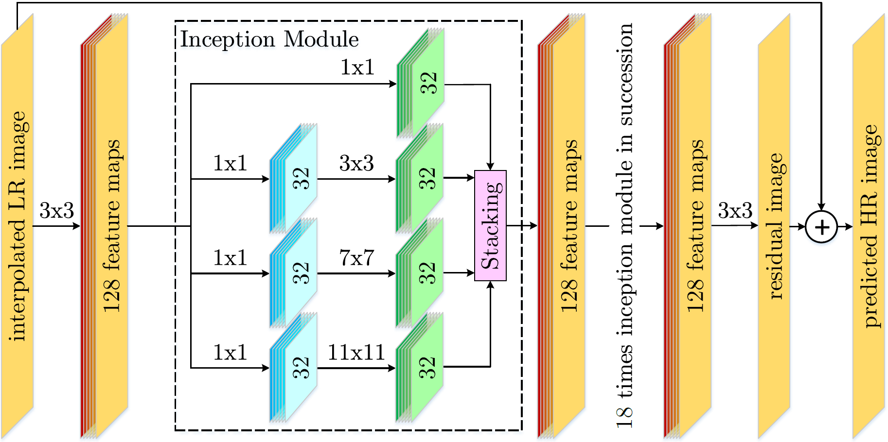
Network Architecture
Proposed super resolution inception (SRINC) architecture: The zero-padded input image is convolved with 128 x 3 x 3 filters in the first layer. After 19 successive inception modules, a last convolutional layer shrinks the feature maps down to the number of output channels, i.e, in our case one (grayscale) channel. Rectified linear units are used between layers except after the final convolution and addition.
Results
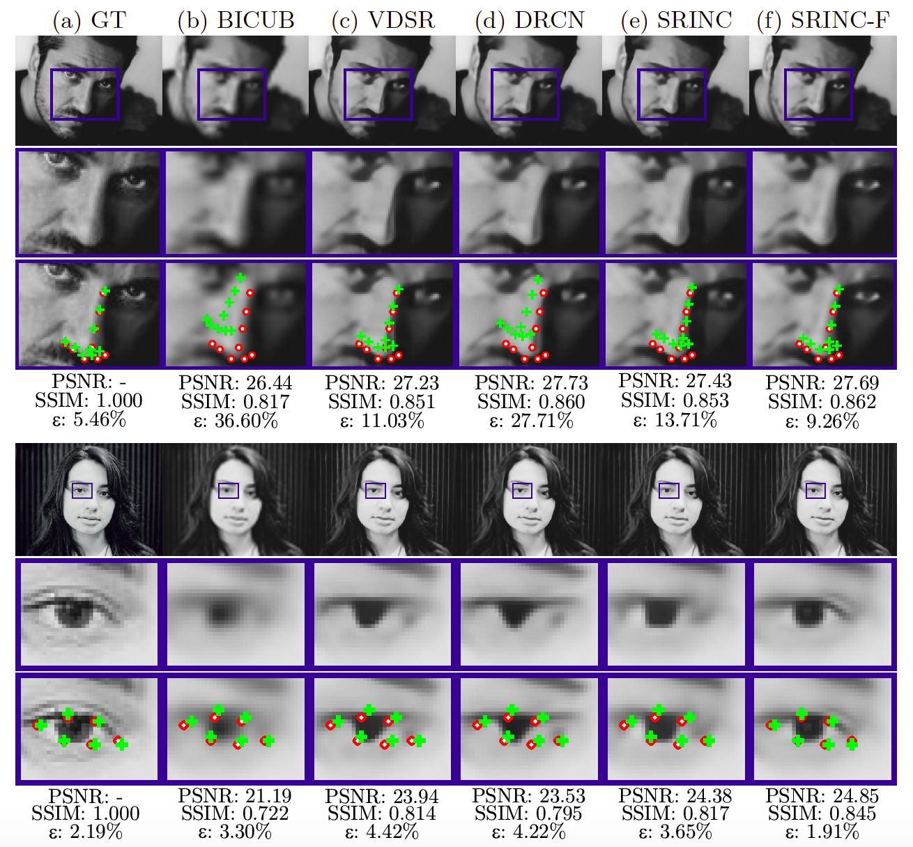
Landmark detection examples for CFSS (top) and TCDCN (bottom) on super resolved low resolution images (x4 scale). Third row also shows ground truth (red dots) and predicted landmarks (green crosses). The provided PSNR and SSIM figures refer to the zoomed patches only.
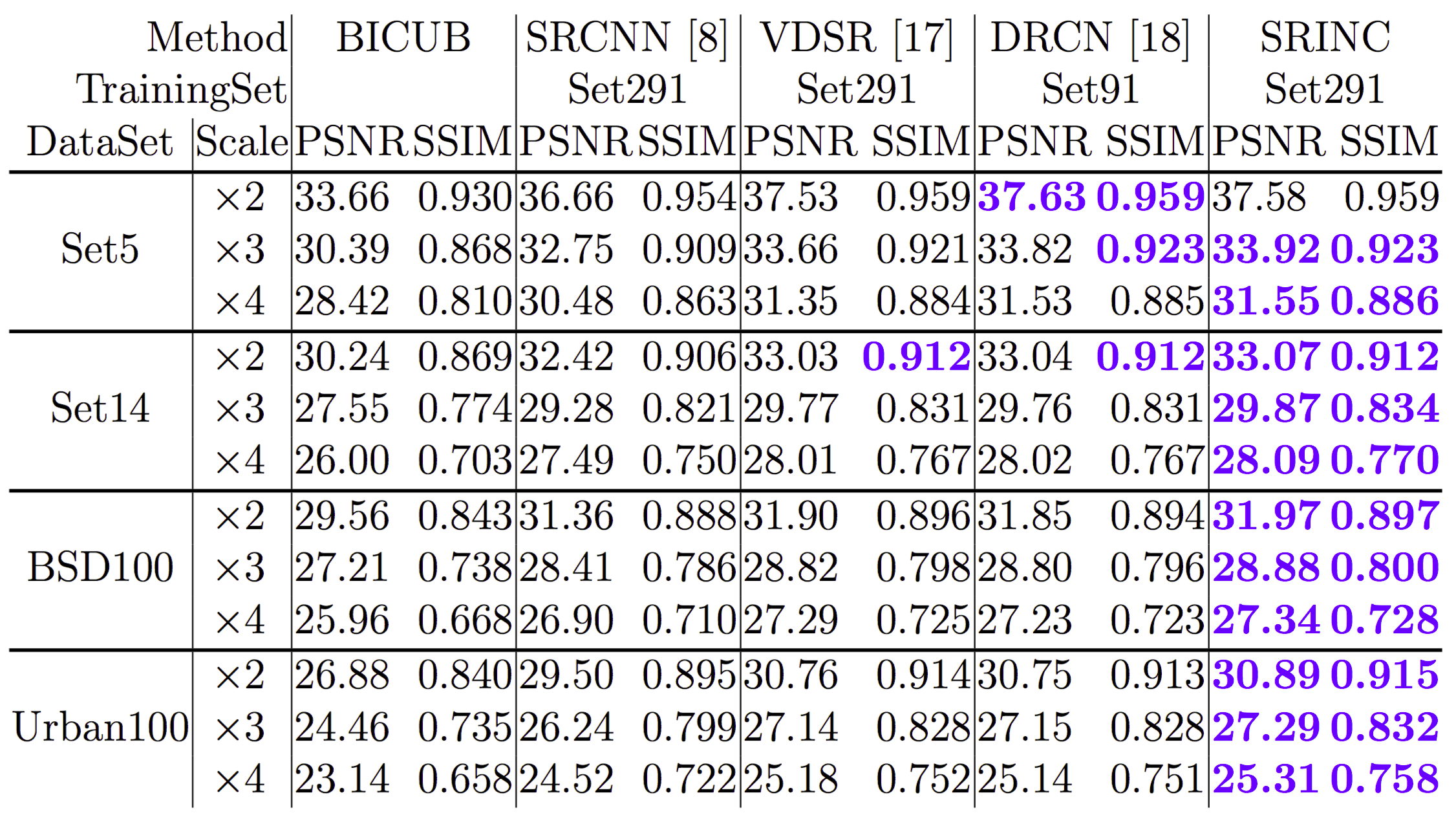
Benchmark
We compared our model (SRINC) to bicubic interpolation, SRCNN, VDSR and DRCN. The results are summarized in the following table:
Download
We provide the following files:
- SRINC Model
- SRINC-F Model (scales 2,3,4)
- SRINC-F Model (scales 8,12,16)
- SRINC-F Model (scales 1,2,3,4)
- SRINC_Main config
- SRINC_Architecture config
- SRINC_Macros config
- SRINC_Inference config
- SRINC_ModelEdit config
- Matlab scripts for patch (de-)composition
- Supplementary material
SRINC.zip (case-sensitive password is: SRINC@MMK)
More details can be found in:
Martin Knoche, Daniel Merget, and Gerhard Rigoll: "Improving Facial Landmark Detection via a Super-Resolution Inception Network", in Proc. German Conference on Pattern Recognition (GCPR), Springer, 2017.
If you use the provided material, please cite our paper!
HowTo use our Code
Pre- & Postprocessing
We extract the Training and Testing Images into Patches before they are used by CNTK. For Training we use 51x51 pixel patches. For Testing we used several sized patches, depending on the dataset. To decompose patches from original images we use the following Matlab code:
PatchDecompose.m
Note that the most right and bottom areas of the image may be duplicated with our method, but we consider the whole image area for the decomposition. For the test data sets there is a fixed overlapping of the patches in order to fully exploit the networks properties. Finally the test set patches are re-composed to get the processed images in the original image dimensions. This helps to process images with arbitrary dimensions in one batch:
PatchCompose.m
When doing inference in CNTK the images are outputted via a simple text file, containing the pixel values row-wise for each image. We convert this file via the following code into an image via Matlab:
for i=1:<Columns in Output Text File>
Img{i} = fliplr(imrotate(reshape(Data(i,:),Config.PatchSize),-90)).*Config.Scale + Config.Bias;
Img{i} = max(16.0, min(235.0 ,Img{i}));
end
Since we normalize the input images inside CNTK to be between 0 and 1, we have to transform it back to the original pixel value space, that is, Config.Scale = 255 . The second line makes sure that the output images have correct pixel intensities in the YCbCr domain.
Training & Inference
After successfully installing Microsoft Cognitive Toolkit (CNTK) you can use our provided configs directly in the command-line window. For example, simply type in cntk.exe configFile="PATH/TO/SRINC_Main.cntk" to start training. Note that you have to adjust all the paths inside the config files to your images and labels first. Before using the inference config you have to edit the model from an input of 51x51 pixel to your desired size of the testing image patches. We used the minimum image dimension of each dataset for the patching and model editing.
Related Downloads
We used different versions of the Microsoft Cognitive Toolkit (CNTK) for development, but the configurations will most likely work on newer releases as well.